Making Control and Machine Learning Systems Safe and Interpretable
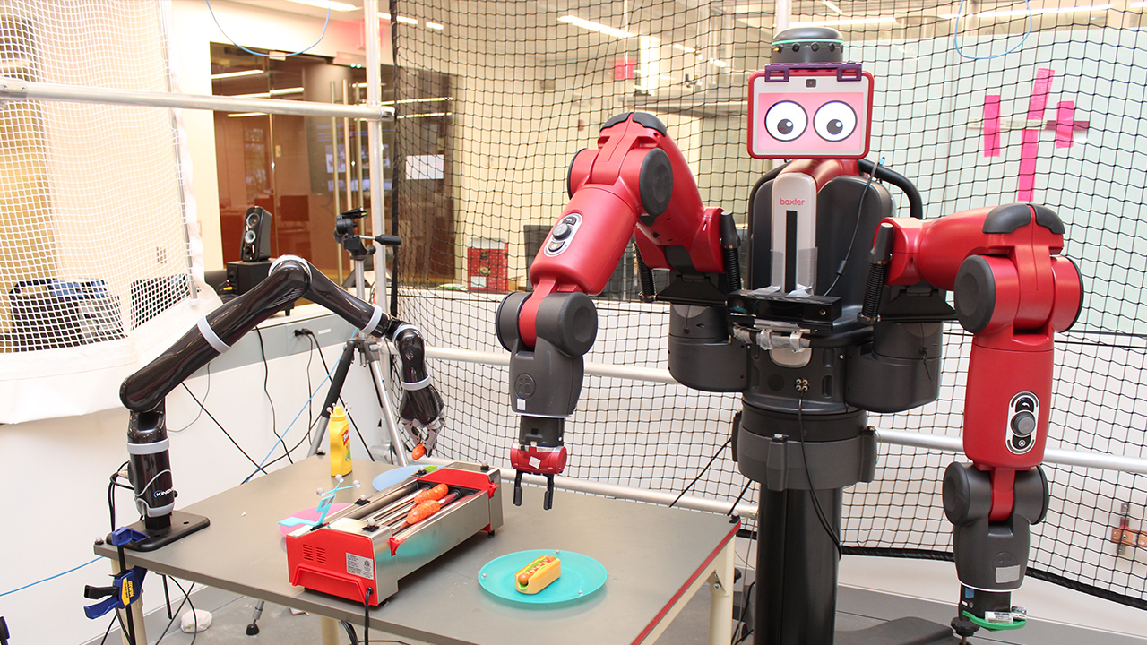
Safe, Interpretable, and Composable Reinforcement Learning for Robotic Manipulation
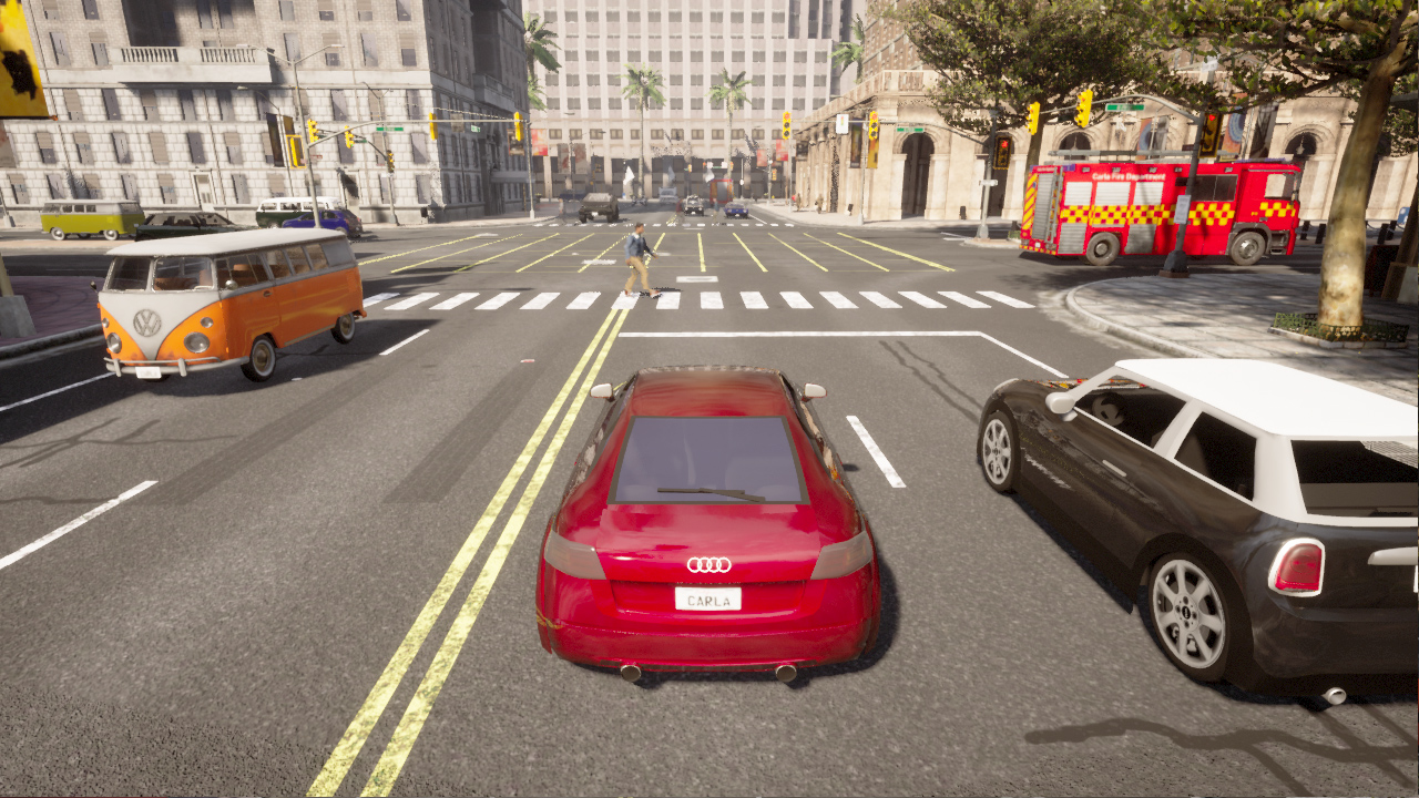
Formal Methods to Comply with Rules of the Road in Autonomous Driving
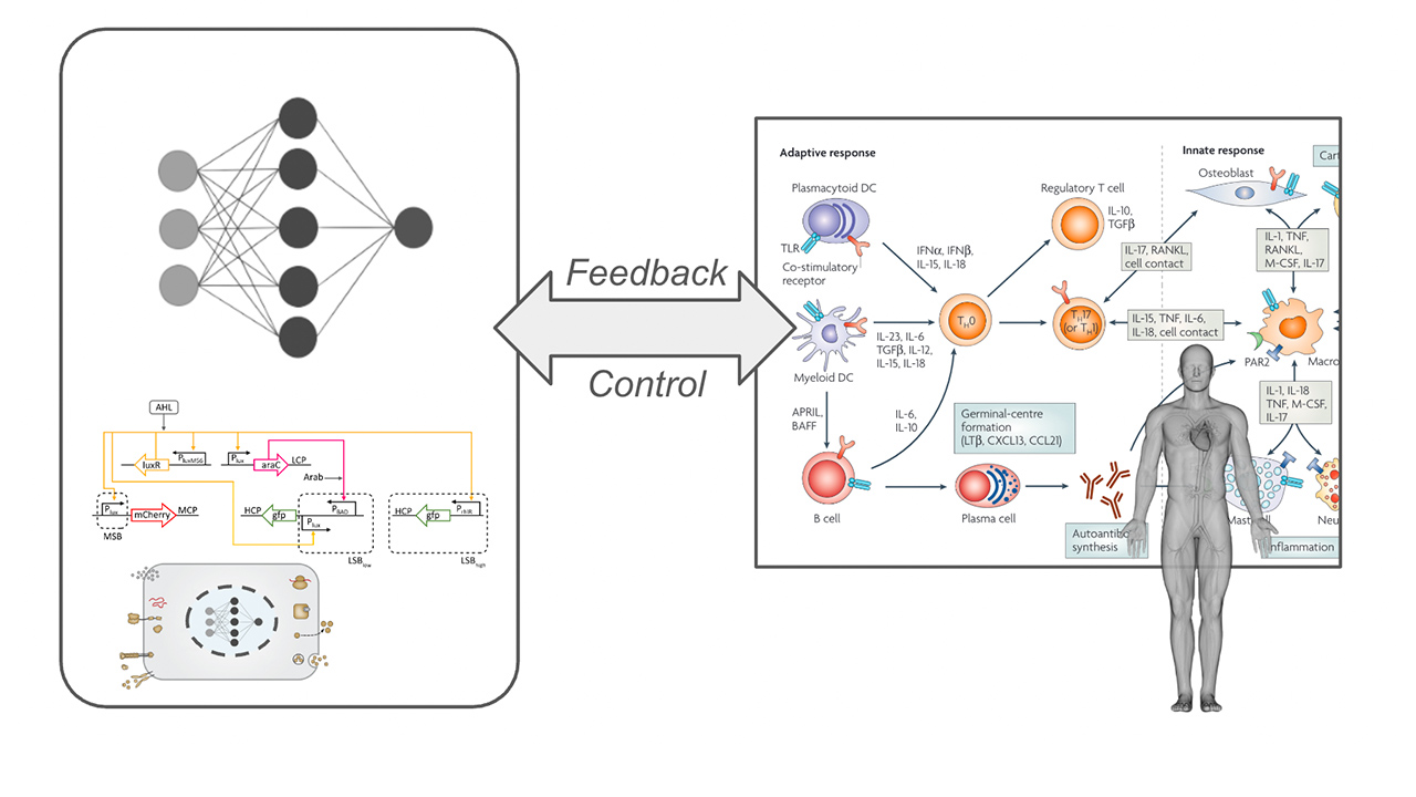
Machine Learning and Control for Synthetic Biology
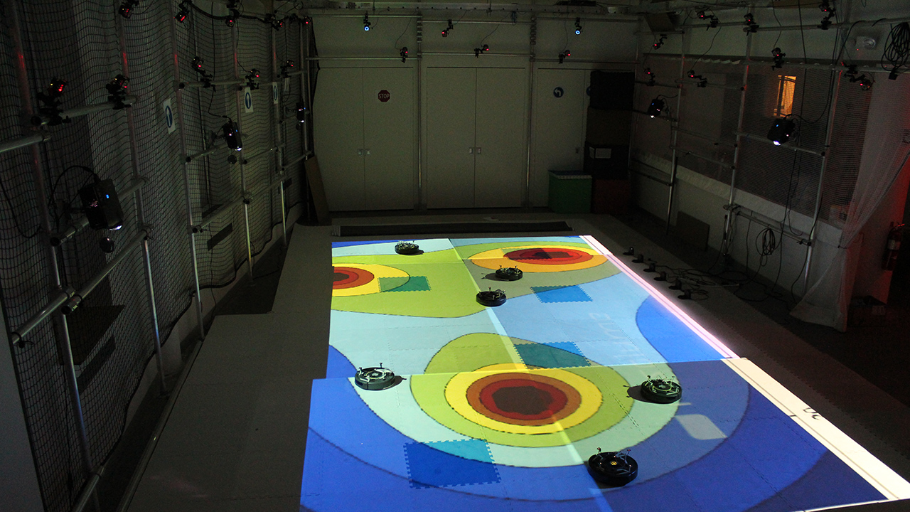
Provably-correct motion planning and control for heterogeneous robotic teams
WELCOME
Calin Belta is the Brendan Iribe Endowed Professor of Electrical and Computer Engineering and Computer Science at the University of Maryland, College Park, where is also part of the Maryland Robotics Center (MRC) and the Institute for Systems Research (ISR). He is also a Research Professor in the College of Engineering at Boston University. His research focuses on dynamics and control theory, with particular emphasis on cyber-physical systems, formal methods, and applications to robotics, autonomous driving, and systems biology.
03/15/24: Calin and Antoine Girard will teach an EECI course “Formal Methods in Control Design: Abstraction, Optimization, and Data-driven Approaches” in Leuven, Belgium, May 27-31, 2024 (see flier for more information, follow this link for registration – select M11)
03/01/24: Calin will be a keynote speaker at ICRA 2024, Yokohama, Japan link
02/26/24: Wenliang Liu defended his PhD thesis and moved on to a position at Amazon
10/11/23: Erfan Aasi defended his PhD thesis and moved to a postdoctoral position at MIT
05/24/23: Max Cohen got the best ME PhD dissertation award!